
An ENTRO (intro) to ENTROpy
Published:
Attribution:
The information in this post is largely derived/inspired from StatQuest with Josh Starmer, who is an amazing YouTuber discussing statistics/data science. I highly recommend checking out his video on Entropy as well.
Introduction
Hello there! Welcome to this post on entropy. Entropy is a crucial concept that appears in various fields, ranging from statistics to machine learning. In this post, we’ll go beyond the formulas to discuss the essence of entropy and what the numbers really mean. Let’s dive in!
What is Entropy?
So, what is entropy? Essentially, entropy is a number that quantifies similarities (or differences). Let’s explore this with an example.
Example
Imagine we have two groups, each consisting of 10 children. In the first group, we have 9 girls and 1 boy. In the second group, there are 5 girls and 5 boys. How would you quantify the similarities of the two groups? Clearly, the first group, with 9 girls and 1 boy, is more “similar” compared to the second group. In the first group, most children are of the same gender, making it more homogenous. In contrast, the second group has an equal distribution of boys and girls, making it less homogenous. This is precisely what entropy can measure.
Intuition
Entropy ranges from 0 to 1. In the second group, where the gender distribution is equal (the most diverse it can get), the entropy is 1. As one gender gradually dominates the population (as in group 1), the entropy decreases towards 0. That’s the basic idea! If you’re only interested in the intuition behind entropy, you can stop here. But why not take a look at the math and explore how the entropy formula is derived?
The Formula of Entropy
From textbooks or online sources, you may know the entropy formula (for a random variable $X$) is:
\[-\sum_x{P(X=x)log[P(X=x)]}\]Hmmm…that looks complicated. I really don’t like reading mathematical equations (nobody does…right?). So, why don’t we simplify it by using the concept of “surprise.” Everyone knows what “surprise” means, right? When an unlikely event happens, we are surprised! But if an event happens frequently, we won’t be surprised at all.
We can apply this concept to the two groups in our example. If we randomly pick a child from the first group, we would be surprised if we picked the boy (because there is only one out of ten children). On the other hand, we wouldn’t be surprised to pick a girl because there are many in group 1. This leads to a crucial relationship:
Surprise is inversely related to probability. A low probability event (like picking a boy in group 1) results in high surprise. A high probability event (like picking a girl in group 1) results in low surprise.
Does this mean we can quantify surprise as the inverse of probability?
\[\frac{1}{\text{probability}}\]While logical, this approach doesn’t work in all cases. For example, consider a group of children consisting only of girls. Picking a child from this group results in no surprise (surprise = 0), but if we use the inverse probability method, surprise would be 1:
\[\text{surprise} = \frac{1}{P(\text{girl})}=\frac{1}{1}=1\]To fix this, we can adjust the formula using a logarithm:
\[\text{surprise} = log(\frac{1}{\text{probability}})\]With this adjustment, picking a girl from an all-girls group results in zero surprise:
\[\text{surprise} = log(\frac{1}{1})=0\]If we try to calculate the surprise of picking a boy from an all-girls group, we get an undefined value:
\[\text{surprise} = log(\frac{1}{0}) = log(1)-log(0)=\text{undefined}\]This undefined result is actually sensible since:
It doesn’t make sense to quantify the surprise of something that never happened before.
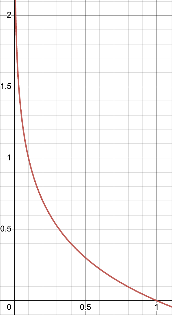
Let’s visualize this relationship. The graph below shows probability on the x-axis and surprise on the y-axis. As probability approaches 1, surprise is 0. As probability approaches 0, surprise increases significantly.
Relating Surprise to Entropy
Now that we understand “surprise” and its formula, let’s relate it back to entropy. Revisit our example of two groups:
| Group | P(Boy) | Boy | P(Girl) | Girl |
|---|---|---|---|---|
| 1 | 0.1 | $\log\left(\frac{1}{0.1}\right) \approx 3.32$ | 0.9 | $\log\left(\frac{1}{0.9}\right) \approx 0.15$ |
| 2 | 0.5 | $\log\left(\frac{1}{0.5}\right) = 1$ | 0.5 | $\log\left(\frac{1}{0.5}\right) = 1$ |
For both groups, we can calculate the expected value of surprise (denoted by $E(surprise)$). Remember, expected value is calculated as:
\[\text{Expected Value of X} = \sum_x{x \cdot P(x)}\]Therefore, we can apply this formula to find the expected value of surprise
\[\text{Expected Value of Surprise} = \sum_x{\text{Surprise of x} \cdot P(x)}\]For the two groups, we can find the expected value of surprise like this:
\[\begin{align*} \text{Expected Surprise of Group 1} &= (3.32)(0.1) + (0.15)(0.9) = 0.47 \\ \text{Expected Surprise of Group 2} &= (1)(0.5) + (1)(0.5) = 1 \end{align*}\]This shouldn’t be too hard to comprehend. But what does this expected value of surprise have anything to do with entropy? If you haven’t already realized, you have just calculated entropy! That’s right! Entropy is really just the expected value of surprise. Let’s put the formula of entropy and the expected value of surprise side by side.
\[\begin{align*} \text{Entropy} &= -\sum_x{P(X=x) \log[P(X=x)]} \\ \text{Expected Value of Surprise} &= \sum_x{\text{Surprise of } x \cdot P(x)} \end{align*}\]These two formulas don’t look the same at all, but wait until I do a little bit of magic.
- Plug in the formula for surprise:
- Expand the log:
- Since $log(1) = 0$:
- Expand the equation:
- Move the negative sign out:
Now, compare this with the entropy formula:
\[\text{Entropy}=-\sum_x{P(X=x)log[P(X=x)]}\]They are the same! In conclusion:
Entropy quantifies similarities (or differences) and is the expected value of surprise. When a group is more homogeneous, entropy is lower, indicating less surprise. When a group is less homogeneous, entropy is higher, indicating more surprise.
Applications of Entropy
- Measuring Uncertainty of Categorical Variables
Entropy is a useful tool for understanding the spread or uncertainty of categorical variables. Unlike variance, which measures how spread out numerical values are, entropy measures how evenly distributed categories are in a dataset.
Think back to our example with two groups of children:
- Group 1: 9 girls and 1 boy.
- Group 2: 5 girls and 5 boys.
In Group 1, most of the children are girls, so the uncertainty is low because it’s highly predictable what gender a randomly picked child will be (mostly girls). This low uncertainty translates to low entropy. In contrast, Group 2 has an equal number of girls and boys, so picking a child randomly is less predictable. This high uncertainty means high entropy.
- Entropy in Decision Trees
Decision trees use entropy to make decisions that lead to more predictable outcomes. The goal is to split the data in a way that makes each group more homogenous, reducing uncertainty.
Returning to our boy and girl example, if we were building a decision tree to predict the gender of a randomly picked child, we might use the existing group split:
- If the child is from Group 1, we would predict “girl” because this group has low entropy (high certainty about the outcome).
- If the child is from Group 2, predicting gender is harder because of the high entropy (more mixed group).
The decision tree would use entropy to identify these splits, choosing conditions that reduce entropy the most to make accurate predictions.
Conclusion
Entropy is a powerful measure of uncertainty, applicable to various scenarios, from understanding the distribution of categories to building predictive models like decision trees. By relating it back to our example of boys and girls, we see how entropy helps quantify how predictable or diverse outcomes are. This understanding allows us to make smarter decisions based on data, whether we are categorizing groups or building complex machine learning models.